Performing data and compatibility analysis
pyddt main goal is to establish a set of systematic procedures for indexing dynamical diffraction peaks and reading their line profile asymmetries, so this approach of using X-ray dynamical diffraction becomes reproducible and transferable.
This last tutorial aims to show the standard procedures implemented into pyddt and analyze two data sets using them.
0. Importing packages
In this tutorial, it’s necessary to use the magic function %matplotlib qt. Using it, matplotlib plots will be opened on an external window from the notebook.
[1]:
%matplotlib qt

import numpy as np
import matplotlib.pyplot as plt

plt.rcParams['font.size'] = '10'

import sys
sys.path.append('path/to/pyddt')

import pyddt
1. Analyzing Renninger scans
1.1 CeFe\(_4\)P\(_{12}\)
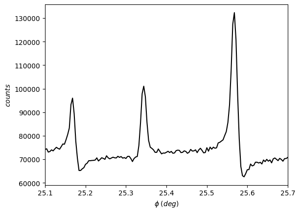
Let’s start by analyzing the scan of the reflection 002, filled skutterudite CeFe\(_{4}\)P\(_{12}\).
X-ray data acquisition was carried out at the Brazilian Synchrotron Light Laboratory (LNLS), bending magnetic beamline XRD2. X-rays of 7105.8 eV.
See Phonon scattering mechanism in thermoelectric materials revised via resonant x-ray dynamical diffraction for a detailed reference.
Creating an expdata object is the first step of data analysis. The necessary inputs are energy value, primary reflection indices, and the filename containing the data.
The data must include the azimuth position and corresponding intensity. For the filled skutterudite, the filename is data_CFP.dat.
[3]:
exp = pyddt.ExpData(7105.8, [0, 0, 2], 'data_CFP.dat')
Once this object was generated, we can visualize the scan.
[13]:
exp.plot()
[13]:
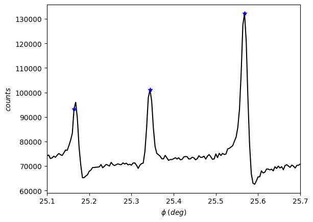
Now, we proceed to find the multiple-diffraction (MD) peaks. You can inform the minimum height to be considered (provide a percentage of the maximum intensity).
For this dataset, 60% is a good choice. Feel free to test other values.
[30]:
exp.peak_finder(0.6)
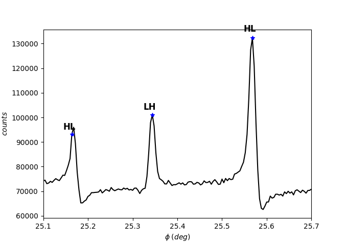
Visualize the scan again to check the selected peaks. You can access the peak positions by using the phi and peaks attributes.
[15]:
exp.plot()
[15]:
[16]:
exp.phi[exp.peaks]
[16]:
array([25.164, 25.344, 25.568])
Our scan is very narrow, so it’s perfectly possible to select the peaks manually. Use the function pyddt.peak_picker() for it.
Also, you can delete peaks by using the function pyddt.review():
To select a peak, stop the mouse over the maximum and press SPACE.
To unselect, stop the mouse over the maximum and press DEL.
Feel free to zoom in or out.
After finishing the selection, press ENTER. Then, close the figure (mouse or press q).
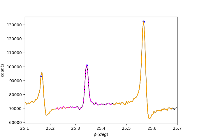
For reading the asymmetries, we fit a superposition of a symmetric peak with a linear slope. This way, it’s necessary to define the fitting region for each selected peak.
The function pyddt.region_of_fit() manually calculates the full width at half maximum \(f\) for each peak, then defines the region of fit as
where \(\phi_{0}\) is the center position and \(n\in \mathcal{Z}\). By default, \(n = 15\).
The calculated regions are exhibited by using flag = 1.
[32]:
exp.region_of_fit(flag=1)
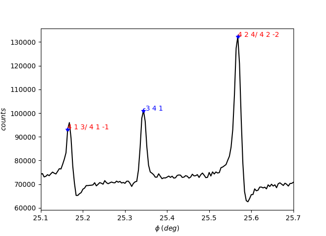
Now, let’s index the MD peaks. To do this, use the pyddt.indexer() function. The secondary reflections are exhibited by using flag = 1.
[33]:
exp.indexer('ce3.in', [1, 1, 0], 50, flag=1)
exp.indexer() arguments:
Structural model (generated in the last tutorial).
Reference direction for the azimuthal rotation
Minimum cutoff for the strength of excitation.
The red color of the 4-beam peaks indicates the in-out geometry of excitation, while blue stands for out-in.
It’s also possible directly index the MD peaks by visualizing \(\omega \times \phi\) graphs. The secondary reflections are shown as hover text by mouse motions.
[ ]:
exp.BC_plot('ce3.in', [1, 1, 0], 50)
You can also access the indexation by calling the index attribute, where \(\pm 1\) stands for the excitation geometry.
[24]:
exp.index
[24]:
array([['1', '4 1 3/ 4 1 -1'],
       ['-1', '-3 4 1'],
       ['1', '4 2 4/ 4 2 -2']], dtype='<U21')
Finally, let’s fit the MD peaks and read their asymmetry.
[34]:
exp.fitter(100)
100%|█████████████████████████████████████████████| 3/3 [00:12<00:00, 4.11s/it]
The slope error is estimated using bootstrap resampling, and the number of resamples is the only argument of exp.fitter() function.
Let’s check the estimated slopes and their errors.
[26]:
exp.slope_data
[26]:
array([[-0.19067251,  0.05101513],
       [ 0.10344877,  0.00676736],
       [-0.20538606,  0.10659999]])
It’s easy to relate the slope sign with the asymmetry type: if negative, the asymmetry is HL (the MD intensity profile has higher/lower shoulders); if positive, it’s LH.
So, the MD peaks observed at 25.16º and 25.57º are HL, while the remaining is LH.
[37]:
exp.asymmetry_assigner(0, 10, flag=1) # flag = 1 to exhibits the asymmetries
The exp.asymmetry_assigner function realizes the asymmetry reading based on the slope sign. Take a look at the API documentation for exploiting the first arguments (cutoff values of \(\bar{S}\) and \(\tau\)).
We have indexed the multiple-diffraction cases and read their asymmetries, so the analysis is finished. Let’s save the results.
[38]:
exp.save()
[38]:
'_E7105.8_G002'
In the current folder, two new files are available: _E7105.8_G002.ext and _E7105.8_G002.red. Take a look at them.
.ext \(\rightarrow\) peak position, hkl, slope, slope error, statistical properties, asymmetry type, and excitation geometry.
.red \(\rightarrow\) hkl, asymmetry, and diffraction geometry (primary indices and energy in 1st line).
1.2 Fe-doped L-asparagine monohydrated
It may seem too much effort to analyze this data using pyddt, since a visual analysis quickly leads to the same conclusions. However, a visual inspection is unworkable as the data set increases. In this situation, pyddt is very helpful.
Another advantage of using pyddt is the analysis of biological materials or X-ray data acquisition on laboratory setups, in which asymmetric profiles aren’t so well-marked.
For illustrating these situations, let’s quickly analyze the scan of the reflection 026, Fe-doped L-asparagine monohydrated.
X-ray data acquisition was carried out at the Sirius, beamline EMA. X-rays of 8048 eV.
[39]:
exp2 = pyddt.ExpData(8048, [0, 2, 6], 'data_lasp.dat')
[40]:
exp2.plot()
[40]:
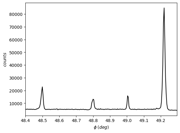
Please, note how the asymmetries are subtle, and a visual asymmetry reading is tricky.
[44]:
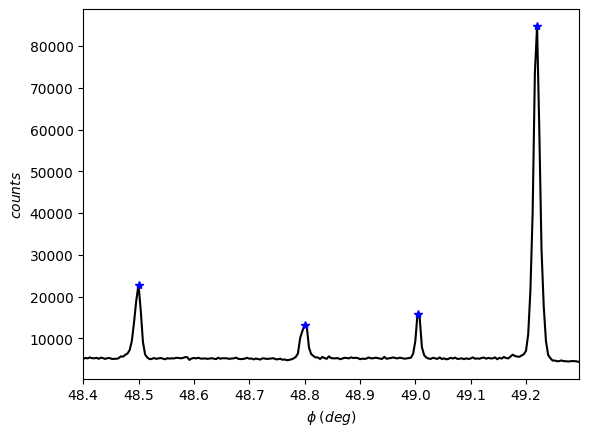
exp2.peak_finder(0.1)
[45]:
exp2.plot()
[45]:
[50]:
exp2.region_of_fit(5, flag=1)
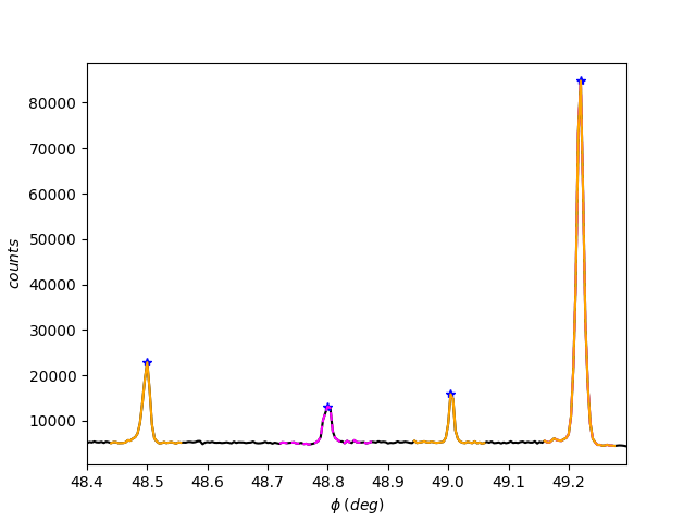
[51]:
exp2.fitter(100)
100%|█████████████████████████████████████████████| 4/4 [00:05<00:00, 1.28s/it]
[52]:
exp2.slope_data
[52]:
array([[-0.17184866,  0.10397331],
       [ 0.15763806,  0.05487308],
       [-0.12616801,  0.08049835],
       [-0.95195789,  0.11601925]])
Compare these values with the estimated for the skutterudite. The ratio slope error/slope is higher now, which indicates low-resolution asymmetries. In this context, pyddt is very helpful.
2. Compatibility analysis
Returning to the filled skutterudite data, we will show how to compare the experimental asymmetries with the predicted structural models.
Within pyddt, the compatibility analysis is performed by the AMD class. The required inputs are the .red file saved after the data analysis and the structural models (created in the last tutorial).
[53]:
amd = pyddt.AMD('_E7105.8_G002.red', ['ce3.in', 'ce4.in'])
Let’s check the experimental asymmetries.
[54]:
amd.asy
[54]:
array(['HL', 'LH', 'HL'], dtype='<U2')
Now, we will use the amd.theoretical_asymmetries() function to calculate the asymmetries predicted by each structural model.
[55]:
amd.theoretical_asymmetries()
[56]:
amd.theo_asy
[56]:
array([[1., 0., 1.],
       [1., 0., 1.]], dtype=float128)
The first line of amd.theo_asy presents the asymmetries calculated by the model ce3.in, where 1 stands for HL and 0 for LH. The asymmetries in the second line were calculated by the model ce4.in.
The multiple-diffraction cases under evaluation don’t allow differentiation of the structural models.
[57]:
amd.hkl
[57]:
array([[ 4.,  1.,  3.],
       [-3.,  4.,  1.],
       [ 4.,  2.,  4.]])
pyddt has other advanced tools for compatibility analysis, which will not be covered in this tutorial. Please, check the API documentation for more details.