Crystallographic calculations

pyddt provides tools for calculating the atomic scattering amplitude, anomalous scattering factors and structure factors of a crystal.

This step-by-step tutorial aims to show some details on pyddt implementation, particularly the interpolation scheme of tabulated scattering amplitudes and the structure factor formula, besides performing these calculations using the package.

1. pyddt implementation

See Computer Simulation Tools for X-ray Analysis: Scattering and Diffraction Methods for detailed reference on X-ray scattering theory.

1.1 Atomic scattering factor and resonance amplitude

For an atom with electronic density \(\rho_{a}(r)\), the coherent scattering intensity is given by

\[I \propto |f_{0}(Q) + f'(E) + if''(E)|^{2}\]

where \(f_{0} = \text{FT}\{\rho_{a}(r)\}\) is the atomic scattering factor and the resonance amplitude \(f'(E) + if''(E)\) is related to the absorption and fluorescence processes. These values are theoretically calculated for all atoms and significant ions.

pyddt uses the tabulated values from the International Tables of Crystallography, considering the linear interpolation of \(f'\) and \(f''\) for energies ranging from 1004.16 eV and 70 keV. The parametric equation

\[f_{0}(\text{sin}\theta/\lambda) = f_{0}(Q/4\pi) = \sum_{i=1}^{4}a_{i}e^{-b_{i}\big(\frac{Q}{4\pi}\big)^{2}} + c\]

is employed for Q < 30 \(\mathring A\)\(^{-1}\). \(a_{i}, b_{i}\) and \(c\) are the Cromer-Mann coefficients.

1.2 Structure factor

Given a crystal, the structure factor of the \(hkl\) lattice plane is calculated by

\[F_{hkl} = \sum_{a}(f_{0} + f' + if'')_{a}C_{a}e^{-M_{a}}e^{2\pi i (hx_{a}+ly_{a}+lz_{a})} = |F_{hkl}|e^{i\delta_{hkl}}\]

where \(a\) summation runs over all atoms inside the unit cell, \(C_{a}\) is the occupancy number, and \((x_{a}, y_{a}, z_{a})\) are the fractional coordinates.

The isotropic Debye-Waller factor

\[M_{a} = 8\pi^{2}\eta_{a}^{2}\bigg(\frac{\text{sin}\theta}{\lambda}^{2}\bigg)\]

represents the crystal disorder, so that \(\eta_{a}\) is the root-mean-square deviation of the \(a\)-th atom in the direction of \(\mathbf{Q}\).

• pyddt current version doesn’t support anisotropic thermal motion.

• The structure file (.in file) must include the B-factors (\(\mathring A\)\(^2\)) of all atoms, defined as

\[B = 8\pi^{2}\eta_{a}^{2}\]

2. Using pyddt

After this brief remarking on the pyddt implementation, let us show how to perform some crystallographic calculations.

2.1 Importing packages

Beyond pyddt, we will also use Numpy for generating arrays and matplotlib for plotting.

import numpy as np
import matplotlib.pyplot as plt

plt.rcParams['font.size'] = '14'

import sys
sys.path.append('path/to/pyddt')

import pyddt

2.2 Atomic scattering factors

Let’s calculate the atomic scattering factor of selenium and reciprocal vector \(Q=8\pi\; (\mathring A\)\(^{-1})\).

pyddt.asfQ('Se', 2)  # Q/4π = 2/Å

array([[4.79787017]])

Try it using different atoms, ions, and \(Q\) values. The asfQ function also works for an array of \(Q\) values.

q = np.linspace(0, 5, 10)  # Q/4π
pyddt.asfQ('Se', q)

array([33.9885    , 16.30767336,  7.86524559,  5.59115665,  4.35547504,
        3.55113219,  3.12239028,  2.93518598,  2.86759017,  2.84728523])

What happens for the Na\(^{3+}\) ion?

pyddt.asfQ('Na3+', 2)

Na3+ is not included in Cromermann factors. Replaced by Na1+

array([[1.03279492]])

pyddt always replaces the ion that isn’t available in the tabulated values with the most similar. A warning always will be show when this kind of replacement happens.

See Analyzing structure factor phases in pure and doped single crystals by synchrotron X-ray Renninger scanning (appendix A) for obtaining the atomic scattering factors of non-tabulated ions by using the available ions.

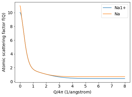
Lastly, let’s visualize the atomic scattering factors as a function of \(Q\) using matplotlib.

q = np.linspace(0, 8, 1000)

fig = plt.figure(figsize=(7, 5))

plt.plot(q, pyddt.asfQ('Na1+', q), '-', label='Na1+')
plt.plot(q, pyddt.asfQ('Na', q), label='Na')

plt.xlabel(r'Q/4$\pi$ (1/angstrom)')
plt.ylabel('Atomic scattering factor f(Q)')
plt.legend()
plt.show()

2.3 Resonance amplitude - anomalous scattering factors

Now, we will show how to obtain the atomic resonance amplitude (also called anomalous scattering factors). The input of aresE function is very similar to the asfQ. For iron and characteristic radiation, one obtains

pyddt.aresE('Fe', 8048)  # 8048 eV

(-1.1306382948756366+3.1972344171411446j)

Considering a range of energies and copper atom,

pyddt.aresE('Cu', np.linspace(2000, 8000, 10))

array([-0.11975181+6.32684898j,  0.09827547+3.9969607j ,
       -0.05817156+2.75911135j, -0.26933609+2.02224386j,
       -0.49158992+1.54844579j, -0.70484541+1.22527238j,
       -0.92480622+0.99511293j, -1.16733754+0.82516188j,
       -1.4683844 +0.69590195j, -1.91835961+0.59518187j])

What happens for an ion? Try to calculate for Fe\(^{2+}\). Is this result physically meaningful?

pyddt.aresE('Fe2+', 8048)  # 8048 eV

0

The answer is no. The resonance amplitude isn’t null for ions, but the tabulated values were only calculated for isolated atoms.

When calculating the structure factors, pyddt will automatically replace the anomalous scattering factor of an ion with the corresponding isolated atom. However, pay attention that this is just an approximation.

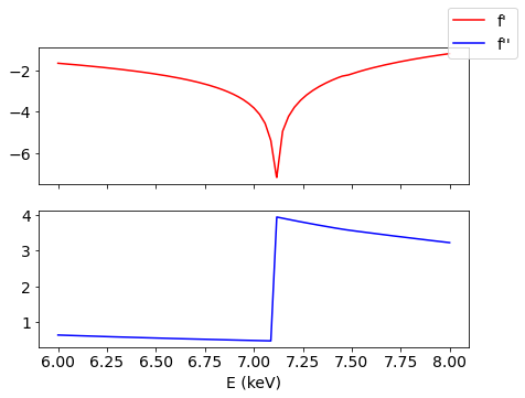
Let’s take a look at the characteristic behavior of resonance amplitude near the Fe absorption edge.

e = np.linspace(6000, 8000, 1000)

fig, (ax1, ax2) = plt.subplots(2, 1, figsize=(7, 5), sharex=True)

ax1.plot(e/1000, np.real(pyddt.aresE('Fe', e)), 'r-', label="f'")
ax2.plot(e/1000, np.imag(pyddt.aresE('Fe', e)), 'b-', label="f''")

plt.xlabel(r'E (keV)')
fig.legend()
plt.show()

2.3 Structure factor

To exemplify the structure factor calculation, let us consider the sodium chloride crystal. You can download its CIF on Materials Project mp-22862.

NaCl.cif

2.3.1 Converting CIF into .in file

The Crystalclass requires an .in file, so we will convert the CIF into the expected format using the pyddt.to_in() function.

pyddt.to_in('NaCl.cif')

In the current folder, two new files are available: NaCl.in and NaCl.struc. Take a look at them.

The .in file presents the atom or ion symbol followed by its fractional coordinates (\(x\), \(y\) and \(z\)), occupancy number and B-factor. The first line shows the lattice parameters (\(a\), \(b\), \(c\), \(\alpha\), \(\beta\) and \(\gamma\)). Meanwhile, the .struc file presents some structural and electronic properties which might be useful for structural modelling.

2.3.2 Crystal object

The next step is generating a crystal object.

nacl = pyddt.Crystal('NaCl.in')

Once this object was created, we can check its lattice and structure.

nacl.structure.lattice

array([ 5.6917,  5.6917,  5.6917, 90.    , 90.    , 90.    ])

nacl.structure.atoms

array(['Na', 'Na', 'Na', 'Na', 'Cl', 'Cl', 'Cl', 'Cl'], dtype='<U32')

nacl.structure.positions

array([[0. , 0. , 0. ],
       [0. , 0.5, 0.5],
       [0.5, 0. , 0.5],
       [0.5, 0.5, 0. ],
       [0.5, 0. , 0. ],
       [0.5, 0.5, 0.5],
       [0. , 0. , 0.5],
       [0. , 0.5, 0. ]])

The bragg() method returns the interplanar distance and Bragg angle from beam energy and the Miller indices.

d, th = nacl.bragg(8048, [1, 0, 0])
print('\nE = 8048 eV - hkl = 100')
print('d = ', np.round(d, 2), 'angstrom')
print('Bragg angle = ', np.round(th, 2), 'deg\n')

E = 8048 eV - hkl = 100
d =  5.69 angstrom
Bragg angle =  7.78 deg

The Fhkl() method returns the complex structure factor. Feel free to try other energy values and hkl indices.

F = nacl.Fhkl(8048, [1, 1, 1])

print(" F = ", np.round(F, 4),
      "\n|F| = ", np.round(np.absolute(F), 4),
      "\nphase = ", np.round(np.angle(F)*180/np.pi, 4), "deg")

 F =  (-18.6152-2.2587j)
|F| =  18.7517
phase =  -173.0818 deg

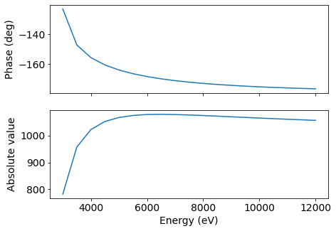
It’s possible to do this calculation for an array of energies or reflections by once.

E = np.arange(3000, 12500, 500)  # eV

fig, (ax1, ax2) = plt.subplots(2, 1, figsize=(7, 5), sharex=True)

ax1.plot(E, np.angle(nacl.Fhkl(E, [1, 1, 1]))*180/np.pi)
ax2.plot(E, np.absolute(nacl.Fhkl(E, [1, 1, 1]))*180/np.pi)

plt.xlabel('Energy (eV)')

ax1.set_ylabel('Phase (deg)')
ax2.set_ylabel('Absolute value')
plt.show()

F = nacl.Fhkl(8048, [[1, 1, 3], [0, 0, 1]])
print('phase = ', *np.angle(F)*180/np.pi, 'degrees')

phase =  -168.935091990334219 90.000000000000003504 degrees

2.3.3 Structure factor list

By the end, let us calculate the structure factor of all reflections.

hkl, f, d = nacl.diffraction(8048)  # Miller indices, structure factors and interplanar distance

hkl

array([[ 0.,  0., -2.],
       [ 0., -2.,  0.],
       [-2.,  0.,  0.],
       ...,
       [-5.,  0., -1.],
       [ 1., -1.,  0.],
       [ 0., -5., -3.]])

d  # angstrom

array([2.84585   , 2.84585   , 2.84585   , ..., 1.11623421, 4.02463967,
       0.9761185 ])

---

In the next tutorial, we will generate structural models by using the Structure class and use them as Crystal objects for planning X-ray dynamical diffraction experiments.